AP Statistics Units Explained: Units 1 to 9 in Plain Language

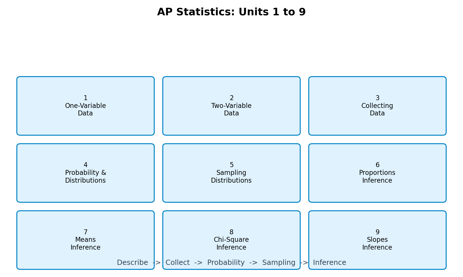
AP Statistics is built from nine units, and each one answers a different question about data. Unit 1 asks what a single set of numbers looks like. Later units ask how samples relate to populations, and whether a pattern is strong enough to believe. If you can see that story, the course feels much less like a list of formulas to memorize.

This guide explains every unit in plain language, names the calculator skill each unit needs, and shows how the units connect.

Unit 1: Exploring One-Variable Data

Unit 1 describes one variable at a time. Students read dot plots, histograms, and box plots, and describe shape, center, and spread. A distribution might be roughly symmetric or skewed, and that shape changes which summary makes sense. The mean and median both describe center, while standard deviation and the interquartile range describe spread. Calculator skills include 1-Var Stats, lists, and graphs, plus the interquartile range rule for outliers.

Unit 2: Exploring Two-Variable Data

Unit 2 looks at relationships between two variables. A scatter plot shows whether two quantities rise together, fall together, or show no pattern. Correlation, written as r, measures the strength and direction of a linear relationship, but it does not prove causation. Regression analysis fits a least-squares line, and residuals show how far each point sits from that line. Calculator skills include scatter plots, LinReg, and residual plots, on a TI-84 Plus, a TI-Nspire, or a free online calculator.

Unit 3: Collecting Data

Unit 3 asks whether the data can be trusted. Students study sampling methods, such as simple random, stratified, and cluster samples, and learn why convenience samples and voluntary response samples can mislead. Experiments add random assignment, control, and replication, so differences in outcomes can be linked to the treatment rather than to hidden variables. Confounding and bias are common traps here. Calculator use is light in this unit, which is itself a lesson: good statistics is not only calculation. The design choices in Unit 3 decide whether later inference is valid.

Unit 4: Probability, Random Variables, and Probability Distributions

Unit 4 introduces probability rules, conditional probability, and random variables. Students learn the mean and standard deviation of a random variable, and that means add while variances add only for independent variables. The normal distribution describes many natural measurements, and students use normalcdf and invNorm for probabilities and percentiles. The binomial distribution models a fixed number of independent trials with the same success probability, using binompdf and binomcdf. These distributions return again in sampling distributions and inference.

Unit 5: Sampling Distributions

Unit 5 is the bridge between probability and inference. A sampling distribution shows what would happen if you took many samples of the same size and calculated a statistic, such as a sample mean or proportion, each time. Its center, spread, and shape show how much sample results naturally vary. The Central Limit Theorem explains why sampling distributions often look approximately normal for large samples, even when the population is not normal. Calculator work here is mostly normal and binomial probability, applied to sample means and proportions.

Unit 6: Inference for Categorical Data: Proportions

Unit 6 is the first full inference unit. Students build confidence intervals for a population proportion and carry out hypothesis testing for a proportion. A confidence interval gives a range of plausible values, while a hypothesis test asks whether data are surprising under a claimed value. Students state hypotheses, check conditions, calculate a test statistic and p-value, and write a conclusion in context. They must not say a test proves a claim; instead, evidence supports or fails to support it. The calculator provides z-interval and z-test output, but interpretation is the student’s job.

Unit 7: Inference for Quantitative Data: Means

Unit 7 applies inference to means. Because population standard deviations are rarely known, students use t-distributions instead of the normal distribution, and degrees of freedom depend on sample size. One-sample and two-sample t-tests, t-intervals, and matched-pairs tests all appear here. Calculator skills include T-Test, 2-SampTTest, and TInterval. The hardest part is often choosing the right procedure and checking conditions, especially for small samples where normality matters more.

Unit 8: Inference for Categorical Data: Chi-Square

Unit 8 uses the chi-square distribution for categorical data. Goodness-of-fit tests ask whether observed counts match an expected pattern, while tests for homogeneity and independence compare distributions across groups or look for an association between two categorical variables. Large gaps between observed and expected counts give a large chi-square statistic and a small p-value.

Unit 9: Inference for Quantitative Data: Slopes

Unit 9 returns to regression from Unit 2, now with inference. Students test whether a population slope is zero and build a confidence interval for a slope. A slope of zero would mean no linear relationship in the population, even if the sample line tilts a little by chance. This unit brings the course together: scatter and residual plots from Unit 2, sampling variation from Unit 5, and hypothesis testing from Units 6 and 7. The calculator’s LinRegTTest gives slope, standard error, test statistic, and p-value, but students must check linear, independent, normal, equal spread, and random conditions first.

How the Units Connect

The units form a chain. Units 1 and 2 describe data. Unit 3 asks whether data can be trusted. Unit 4 gives probability tools, and Unit 5 shows how samples vary. Units 6 through 9 then use those tools for inferences about proportions, means, chi-square tables, and slopes.

Frequently Asked Questions

Which AP Statistics unit is the hardest?

Many students find Unit 5, sampling distributions, or Unit 9, inference for slopes, hardest, because both combine earlier ideas. Revisiting probability and scatter plots usually makes both easier.

How much of the exam covers each unit?

Exam weight varies by year, but Units 1, 3, 4, 6, and 7 together carry a large share. No unit can safely be skipped, and free-response questions often combine units, for example asking for a graph, a probability, and an inference conclusion in one problem.

What calculator skills do I need for AP Statistics?

The core skills are 1-Var Stats, scatter plots and regression, normalcdf and invNorm, binompdf and binomcdf, t-tests and t-intervals, chi-square tests, and LinRegTTest. Practise them until the menus feel routine, so exam time goes to reasoning.

Do I need to memorize every formula?

The AP Statistics exam provides a formula sheet, so the goal is knowing when to use each formula, not memorizing every symbol. Students still need conditions, interpretations, and how to read calculator output.

Conclusion

AP Statistics units tell one story: describe data carefully, collect it well, understand how samples vary, then make careful inferences. Practise the calculator skill for each unit, and write conclusions in plain language and in context. For quick checks on normal probabilities, binomial probabilities, t-tests, chi-square tests, and regression, try the free Ap Stats Calculator at www.apstatscalculator.com.

AP is a trademark of the College Board, which was not involved in the production of this site.